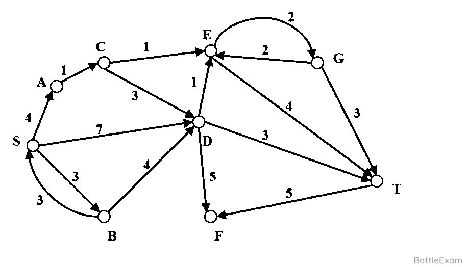
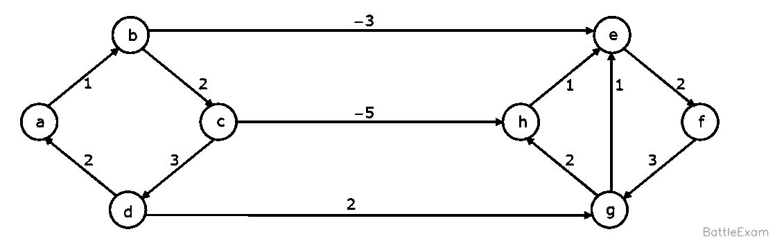
📘 Shortest Path – Concept Summary
### 1. Foundational Definitions and Taxonomy
In the architecture of graph theory and competitive frameworks like the GATE CSE exam, shortest path algorithms are strategically vital. They provide the computational backbone for network routing, logistics optimization, and pathfinding in road networks. Understanding these algorithms is not merely about finding a route but about optimizing cost and resources within complex systems.
**Key Concepts:**
- **Shortest Path**: A path between two vertices where the sum of the weights of its constituent edges is minimized.
- **Weighted vs. Unweighted Graphs**: In weighted graphs, each edge has a numerical cost; in unweighted graphs, every edge is treated as having a uniform cost (usually 1).
- **Directed vs. Undirected Graphs**: Directed graphs (using "arcs") restrict traversal to specific directions, while undirected graphs allow bidirectional travel.
- **Single-Source vs. All-Pairs**: Single-Source Shortest Path (SSSP) finds the distance from one root to all other nodes. All-Pairs Shortest Path (APSP) computes the minimum distance between every possible pair of vertices ($O(V^3)$ typically).
- **Negative Edges**: Edges with a weight less than zero. These can reduce the total path cost as they are traversed.
- **Negative Cycles**: A cycle where the total sum of edge weights is negative. In such cases, a shortest path is often undefined because one could traverse the cycle infinitely to decrease the path cost to $-\infty$.
**Impact of Negative Edge Weights: A Numerical Example**
Negative weights complicate path calculations by potentially making longer paths (in terms of edge count) cheaper than direct paths.
*Input*: $V=5$, Edges = `[[0, 1, 5], [1, 2, 1], [1, 3, 2], [2, 4, 1], [4, 3, -1]]`.
- Path $0 \rightarrow 1 \rightarrow 3$: Weight = $5 + 2 = 7$.
- Path $0 \rightarrow 1 \rightarrow 2 \rightarrow 4 \rightarrow 3$: Weight = $5 + 1 + 1 + (-1) = 6$.
- *Conclusion*: Even though the second path uses more edges, the negative edge $(4, 3)$ makes it the optimal choice.
### 2. The Core Mechanics: Relaxation and Algorithmic Paradigm
The "Relaxation" principle serves as the universal building block for shortest path algorithms. Strategically, it allows an algorithm to move from an initial estimate of infinity toward the true optimal distance by iteratively refining path costs.
**Relaxation Intuition:**
The logic is simple: If the current known distance to a node $v$ is greater than the distance to node $u$ plus the weight of the edge $(u, v)$, we update the distance to $v$.
*Update Rule*: `if dist[v] > dist[u] + weight(u, v) then dist[v] = dist[u] + weight(u, v)`. This update is "safe" because it only ever decreases the distance estimate, moving it closer to the actual shortest path value. Once no more edges can be relaxed, the graph has reached a state of stability.
**Algorithmic Paradigms:**
The choice between greedy and dynamic programming (DP) involves a fundamental trade-off between speed and the ability to handle arbitrary edge weights:
- **Greedy (Dijkstra)**: Selects the "local" best option (minimum distance) at each step. It is highly efficient but assumes that once a node is finalized, its distance is permanent.
- **Dynamic Programming (Bellman-Ford, Floyd-Warshall)**: Computes paths in a bottom-up manner (e.g., paths with at most $k$ edges). This allows the algorithm to handle negative weights and detect negative cycles by checking if a $V$-th edge can still reduce the path cost.
### 3. Key Mathematical and Logical Properties
Shortest path problems rely on the Optimal Substructure property: if a shortest path from A to C passes through B, then the sub-paths A $\rightarrow$ B and B $\rightarrow$ C must also be shortest paths.
> **Revision Cheat-Box:**
> - **Optimal Substructure**: Shortest paths are composed of shortest sub-paths. This property is necessary for DP/Greedy solutions. Note: The Longest Path problem lacks this property in general graphs, making it NP-Hard.
> - **Triangle Inequality**: For any edge $(u, v)$, the shortest distance satisfies $dist(s, v) \le dist(s, u) + weight(u, v)$.
> - **Reachability**: If no path exists from source $s$ to node $v$, the distance is defined as $\infty$ (specifically $10^8$ in standard implementation practice).
> **GATE Observation: MST vs. SPT (Adding a constant $\alpha$ to all edge weights)**
> - **Minimum Spanning Tree (MST)**: Every MST remains an MST because the relative order and number of edges in a tree are fixed.
> - **Shortest Path Tree (SPT)**: SPs may change. Adding $\alpha$ penalizes paths with more edges more heavily than those with fewer edges.
> - **Total Weight**: A Shortest Path Tree (SPT) minimizes individual distances from a source; its total edge weight is not necessarily minimized and is generally higher than that of an MST.
### 4. Breadth-First Search (BFS) for Unweighted Graphs
For graphs where all edges have equal weight, BFS is the most efficient choice. It finds the shortest path in terms of the minimum number of edges.
**Pseudocode:**
```javascript
Initialize dist[all] = 10^8, dist[source] = 0
Queue q.enqueue(source)
while q is not empty:
u = q.dequeue()
for each neighbor v of u:
if dist[v] == 10^8: // Unvisited
dist[v] = dist[u] + 1
q.enqueue(v)
```
**Complexity and Logic:**
BFS uses level-order traversal, which naturally discovers nodes in increasing order of their distance. The time complexity is $O(V+E)$.
> **Common Trap**: BFS only minimizes the number of edges. Never apply BFS to a weighted graph to find the minimum weight path unless all weights are 1 (or equal). For weights of $0$ and $1$, use $0\text{-}1$ BFS with a double-ended queue.
### 5. Dijkstra’s Algorithm: The Greedy Workhorse
Dijkstra's is the dominant SSSP algorithm for non-negative weights. It utilizes a greedy approach to finalize the distance to the "closest" unvisited node.
**Step-by-Step Intuition:**
1. **Initialize**: Source distance = 0, others = $10^8$. Use a Min-Heap (Priority Queue).
2. **Select**: Extract the vertex $u$ with the minimum $dist[u]$.
3. **Relax**: Update neighbors of $u$. If $dist[v] > dist[u] + w(u,v)$, update $dist[v]$ and the heap.
**Why Negative Edges Fail (The One-Pass Greedy Failure):**
Dijkstra's is a one-pass greedy algorithm. Once a node is extracted from the Priority Queue, it is marked "visited" and its distance is finalized. If a negative edge is found later, it could reveal a shorter path to an already "visited" node. Because Dijkstra doesn't revisit nodes, it cannot account for this domino effect, leading to incorrect results.
**Implementation Comparison:**
| Implementation | Complexity | Best Use Case |
| :--- | :--- | :--- |
| **Adjacency Matrix** | $O(V^2)$ | Dense Graphs |
| **Adjacency List + Min-Heap** | $O(E log V)$ | Sparse Graphs |
| **Fibonacci Heap** | $O(E + V log V)$ | Theoretical Best / Conceptual Questions |
> **GATE Trap**: Dijkstra's may work on specific graphs with negative edges by chance, but it is never guaranteed.
### 6. Bellman-Ford Algorithm: Handling Negative Weights
Bellman-Ford is the standard for graphs with arbitrary weights. Its strategic value lies in its ability to detect negative cycles.
**Key Mechanics:**
- **Principle of $V-1$ Relaxations**: A simple shortest path in a graph with $V$ vertices can have at most $V-1$ edges. Relaxing all edges $V-1$ times ensures the shortest path information has propagated to all nodes.
- **Negative Cycle Detection**: If a $V$-th iteration results in a distance update, a negative cycle exists.
- **Exam Implementation**: If a negative cycle is detected, the algorithm should return -1.
- **Unreachable Nodes**: For any node $v$ where no path exists from source, $dist[v]$ remains $10^8$.
- **Complexity**: $O(V \cdot E)$. It is slower than Dijkstra but required for arbitrary weights.
### 7. Floyd-Warshall Algorithm: All-Pairs DP
When the shortest path between every pair is required, Floyd-Warshall uses a DP approach suited for dense graphs.
**DP Transition Relation:**
$dist[i][j] = \min(dist[i][j], dist[i][k] + dist[k][j])$. This checks if passing through an intermediate vertex $k$ provides a shorter route.
**Complexity and Cycles:**
- **Time Complexity**: $O(V^3)$.
- **Cycle Detection**: If any diagonal element $dist[i][i] < 0$, a negative cycle exists.
### 8. Comparative Analysis and Strategy Matrix
| Algorithm | Graph Type | Negative Edges? | Negative Cycles? | Complexity | Strategy |
| :--- | :--- | :--- | :--- | :--- | :--- |
| **BFS** | Unweighted | No | No | $O(V+E)$ | Level-Order |
| **Dijkstra** | Weighted | No | No | $O(E \log V)$ | Greedy |
| **Bellman-Ford** | Weighted | Yes | Returns -1 | $O(VE)$ | DP |
| **Floyd-Warshall** | All-Pairs | Yes | Detects | $O(V^3)$ | DP |
| **DAG-Shortest Path** | Directed Acyclic | Yes | N/A | $O(V+E)$ | Topo Sort |
### 9. In-Depth Complexity and Graph Structure Impact
- **Dense Graphs ($E \approx V^2$)**: Floyd-Warshall or Matrix-based Dijkstra.
- **Sparse Graphs ($E \approx V$)**: Heap-based Dijkstra or Johnson’s Algorithm.
- **Directed Acyclic Graphs (DAGs)**: Shortest and Longest Paths can be found in $O(V+E)$ linear time using Topological Sort. While Longest Path is NP-Hard for general graphs, the acyclic property of DAGs allows linear-time relaxation.
### 10. Problem Identification and Exam Heuristics
**Keyword-to-Algorithm Map:**
- "Minimum cost" + "Positive weights" $\rightarrow$ Dijkstra.
- "Arbitrary weights" + "Detect cycle" $\rightarrow$ Bellman-Ford.
- "Between all pairs" $\rightarrow$ Floyd-Warshall.
- "Unweighted" or "Minimum steps in a maze/grid" $\rightarrow$ BFS.
**GATE Tricks:**
- **Snake and Ladder / Knight Moves**: Always interpret as BFS on an unweighted graph.
- **Disconnected Graphs**: Ensure distance is initialized to $10^8$.
### 11. Classic GATE Scenario Analysis
- **Network Routing**: OSPF uses Dijkstra's; RIP uses Bellman-Ford logic (Distance Vector).
- **Maze Navigation**: BFS for shortest path in steps (e.g., minimum knight moves to reach a target cell).
- **Shortest Path in DAG**: Process vertices in Topological Order; total time $O(V+E)$.
### 12. Advanced Conceptual Extensions
- **Johnson’s Algorithm**: Solves APSP in sparse graphs by re-weighting edges (using Bellman-Ford) to eliminate negatives, then running Dijkstra from every node. Complexity: $O(VE + V^2 \log V)$.
- **0–1 BFS**: Used when weights are only 0 or 1. Use a deque: push 0-weight edges to the front and 1-weight edges to the back.
- **Difference Constraints**: Solving a system of inequalities $x_j - x_i \le w_{ij}$ using Bellman-Ford on a constraint graph.
### 13. Fast Revision: The "Shortest Path" Cheat Sheet
- **Dijkstra**: Greedy. No negative edges. $O(E \log V)$.
- **Bellman-Ford**: DP. $V-1$ iterations. Returns -1 for negative cycles. $O(VE)$.
- **Floyd-Warshall**: All-Pairs. $O(V^3)$. Check $dist[i][i]$ for cycles.
- **DAG**: Topological Sort. Linear time $O(V+E)$. Works for both Shortest and Longest paths.
- **MST vs SPT**: MST minimizes total tree weight. SPT minimizes path from source. Adding a constant weight $\alpha$ to all edges preserves MST but changes SPT.
- **The Infinity Standard**: For unreachable vertices, use $10^8$.